Probability and Expected Value - A Dice Toss Experiment
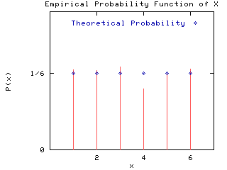
Suppose the random variable X is the number resulting from the toss of a fair die. The probability function is:
PX(x) = P(X=x) = 1/6
for x = 1,2,3,4,5,6
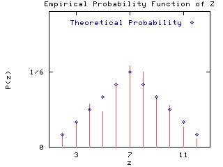
Let the random variable Y be the number resulting from the toss of a second die. The sum of the two faces is Z=X+Y. The probability function of Z is:
  z     2    3    4    5    6    7    8    9   10   11   12
 P(z)  1/36 2/36 3/36 4/36 5/36 6/36 5/36 4/36 3/36 2/36 1/36
The expected value of Z is:
E(Z) =  z P(z)
= (2)(1/36) + (3)(2/36) + ... + (12)(1/36)
= 7
The probability function can be derived empirically by using relative frequencies to estimate probabilities. That is, if two dice are tossed a large number of times, the relative frequencies for each possible outcome should be close to the theoretical probabilities given above. The average over all dice tosses of the sum of the two dice faces should be close to the expected value. That is, expectation has the interpretation as the average value of a random variable over a large number of trials.
The dice toss experiment can be simulated with a computer program. A random number generator is used to simulate the repeated tosses of two dice. Relative frequencies and summary statistics are then calculated. This is shown with the SHAZAM commands:
* Set the number of tosses GEN1 N=500 SAMPLE 1 N * Toss 2 dice GENR x=INT(UNI(6)) + 1 GENR y=INT(UNI(6)) + 1 STAT x y / PFREQ * Calculate the sum GENR sum=x+y STAT sum / PFREQ STOP |
On the GENR command the UNI(b) function
is used to generate a uniform random number x such that
0 < x < b.
The INT(a) function returns the integer part of a.
Therefore, the function INT(UNI(6)) will generate a number
that is one of 0, 1, 2, 3, 4 or 5 (each is equally likely).
In the above commands the number of trials is set to 500. This choice is arbitrary. An increase in the number of trials will require more computing time. But with high speed personal computers this may not be a concern. A choice of 10,000 or 20,000 for the number of trials will give greater accuracy.
The SHAZAM output can be viewed.
Note that, since the numerical results depend on random numbers,
different runs of the program will give different answers.
To obtain the same random numbers in different runs the command
SET RANFIX should be placed at the top of the SHAZAM
commands.
The figures below give plots of the probability functions for X and Z.
 [SHAZAM Guide home]
SHAZAM output - Dice Toss Experiment
|_* Set the number of tosses
|_GEN1 N=500
|_SAMPLE 1 N
|_* Toss 2 dice
|_GENR x=INT(UNI(6)) + 1
|_GENR y=INT(UNI(6)) + 1

|_STAT x y / PFREQ
NAME        N   MEAN        ST. DEV      VARIANCE     MINIMUM      MAXIMUM
X          500   3.4720       1.7411       3.0313       1.0000       6.0000
Y          500   3.5100       1.6827       2.8316       1.0000       6.0000

 VARIABLE = X
         VALUE       FREQUENCY    PERCENT   CUMULATIVE
     1.0000000            87      0.17400   0.17400
     2.0000000            86      0.17200   0.34600
     3.0000000            90      0.18000   0.52600
     4.0000000            66      0.13200   0.65800
     5.0000000            83      0.16600   0.82400
     6.0000000            88      0.17600   1.00000

MEDIAN =    3.0000
LOWER 25%=   2.0000     UPPER 25%=   5.0000     INTERQUARTILE RANGE=  3.000
MODE =    3.0000     WITH       90 OBSERVATIONS

 VARIABLE = Y
         VALUE       FREQUENCY    PERCENT   CUMULATIVE
     1.0000000            80      0.16000   0.16000
     2.0000000            80      0.16000   0.32000
     3.0000000            92      0.18400   0.50400
     4.0000000            78      0.15600   0.66000
     5.0000000            93      0.18600   0.84600
     6.0000000            77      0.15400   1.00000

MEDIAN =    3.0000
LOWER 25%=   2.0000     UPPER 25%=   5.0000     INTERQUARTILE RANGE=  3.000
MODE =    5.0000     WITH       93 OBSERVATIONS

|_* Calculate the sum
|_GENR sum=x+y
|_STAT sum / PFREQ
NAME        N   MEAN        ST. DEV      VARIANCE     MINIMUM      MAXIMUM
SUM        500   6.9820       2.3445       5.4967       2.0000       12.000

 VARIABLE = SUM
         VALUE       FREQUENCY    PERCENT   CUMULATIVE
     2.0000000            14      0.02800   0.02800
     3.0000000            28      0.05600   0.08400
     4.0000000            48      0.09600   0.18000
     5.0000000            39      0.07800   0.25800
     6.0000000            67      0.13400   0.39200
     7.0000000            90      0.18000   0.57200
     8.0000000            83      0.16600   0.73800
     9.0000000            54      0.10800   0.84600
     10.000000            46      0.09200   0.93800
     11.000000            22      0.04400   0.98200
     12.000000             9      0.01800   1.00000

MEDIAN =    7.0000
LOWER 25%=   5.0000     UPPER 25%=   9.0000     INTERQUARTILE RANGE=  4.000
MODE =    7.0000     WITH       90 OBSERVATIONS
|_STOP
[SHAZAM Guide home]