The Distribution of the Durbin-Watson Test Statistic Consider a linear regression equation where the equation errors follow an AR(1) error process:       t = t-1 + vt     with   -1 < < 1 For a test of postive autocorrelation in the errors the null and alternative hypotheses are:       H0: = 0     against   H1: > 0 A test of negatively autocorrelated errors tests:       H0: = 0     against   H1: < 0 The Durbin-Watson test statistic is calculated from the OLS estimated residuals êt as:       d = tN=2 (êt - êt-1)2 / tN=1 êt2 The d-statistic has values in the range [0,4]. Low values of d are in the region for positive autocorrelation. Values of d that tend towards 4 are in the region for negative autocorrelation. (See textbooks for further discussion). Therefore, for a one-tailed test against postive autocorrelation, at a 5% significance level the null is rejected if         d < dcp where dcp is a critical value such that:         P(d < dcp) = 0.05 For a one-tailed test against negative autocorrelation, at a 5% level the null is rejected if         d > dcn     where         P(d > dcn) = 0.05     or         P(d < dcn) = 0.95 A complication is that the probability distribution of d depends on the data matrix X. Therefore, it is not possible to tabulate critical values that can be applied to all models. For a specific model, SHAZAM can compute a p-value for the Durbin-Watson test. This is obtained with the DWPVALUE option on the OLS command. With high speed personal computers the computation is fast for most models. An example of the probability distribution of d can be shown with the Theil textile data set. 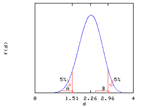The linear regression equation is:       CONSUMEt = 0 + 1 INCOMEt + 2 PRICEt + t Computer simulation was used to generate the probability distribution of d under the null hypothesis of no autocorrelation when the explanatory variables are INCOME and PRICE (and a constant). The SHAZAM commands are available. The result is shown in the figure below. For this example, the mean of the distribution of d is 2.26. The 5% critical value for a one-tailed test against positive autocorrelation is 1.506. The 5% critical value for a one-tailed test against negative autocorrelation is 2.964. These critical values can be compared with the lower bound dl and upper bound du critical values that are tabulated in the Appendixes of econometrics textbooks (computation of the critical values is presented in Savin and White [1977]). In the above figure region A is: [dl, du] = [1.015, 1.536] and region B is: [4-du, 4-dl] = [2.464, 2.985] It can be seen that the 5% critical value of 1.506 is very close to the upper bound du. This conforms to the following comment by Theil [1971, p. 201]. ... the upper bound du is approximately equal to the true significance limit in all those cases in which the behavior of the explanatory variables is smooth in the sense that their first and second differences are small compared with the range of the corresponding variable itself. Many economic time series are characterized by considerable inertia, so that this condition is then at least approximately satisfied. ... However, note that the smoothness condition is not satisfied by dummy variables, which jump from zero to one and vice versa, nor by most of the regressions that are formulated in terms of the first differences of the original variables. Large Samples An artificial data set with an X matrix of dimension (500 x 5) was generated. The OLS / DWPVALUE command in SHAZAM required a memory allocation of PAR=2005. With a Pentium 200Mhz computer running the Linux operating system the calculations took 25 seconds. However, Harvey [1990, p. 201] notes that, for large sample sizes, d is approximately normally distributed with mean 2 and variance 4/N. Using this result, with N=500, the 5% critical value for a one-tailed test against positive autocorrelation is 1.85. This critical value can be computed with the SHAZAM commands: SAMPLE 1 1 GEN1 V=4/500 GEN1 P=0.95 DISTRIB P / TYPE=NORMAL INVERSE MEAN=2 VAR=V STOP References Durbin, J. and Watson, G.S., "Testing for Serial Correlation in Least Squares Regression I", Biometrika, Vol. 37, 1950, pp. 409-428. Durbin, J. and Watson, G.S., "Testing for Serial Correlation in Least Squares Regression II", Biometrika, Vol. 38, 1951, pp. 159-178. Harvey, A.C., The Econometric Analysis of Time Series, Second Edition, MIT Press, 1990. Savin, N.E. and White, K.J., "The Durbin-Watson Test for Serial Correlation with Extreme Sample Sizes or Many Regressors", Econometrica, Vol. 45, 1977, pp. 1989-1996. Theil, H., Principles of Econometrics, Wiley, 1971. [SHAZAM Guide home] SHAZAM commands ?DEMO SET RANFIX NOOUTPUT NODOECHO SET MAXCOL=2010 * Set the number of replications GEN1 NREP=2000 * Set the step-size for numerical differentiation GEN1 STEP=0.001 * Set the "true model". OLS CONSUME INCOME PRICE / PREDICT=YHAT GEN1 SIG=SQRT($SIG2) * Get eigenvalues required for the Imhof routine GENR ONE=1 COPY INCOME PRICE ONE X MATRIX M=IDEN(17)-X*INV(X'X)*X' * Generate the A matrix GENR D=2 IF (TIME(0).EQ.1) D=1 IF (TIME(0).EQ.17) D=1 MATRIX A=IDEN(17,2) MATRIX A=-(A+A')+DIAG(D) MATRIX MA=M*A MATRIX EVAL=EIGVAL(MA) GEN1 CRITL=0 GEN1 CRITU=4 GEN1 CRITM=0 DIM TEST NREP PDF NREP DO #=1,NREP * The null hypothesis is no autocorrelation GENR E=NOR(SIG) GENR Y=YHAT+E OLS Y INCOME PRICE / RSTAT GEN1 DW=$DW GEN1 TEST:#=DW DIST DW / EIGENVAL=EVAL TYPE=IMHOF NEIGEN=14 GEN1 CDF=$CDF IF1 ((CDF.LT.0.05) .AND. (DW.GT.CRITL)) CRITL=DW IF1 ((CDF.LT.0.50) .AND. (DW.GT.CRITM)) CRITM=DW IF1 ((CDF.GT.0.95) .AND. (DW.LT.CRITU)) CRITU=DW GEN1 DW=DW+STEP DIST DW / EIGENVAL=EVAL TYPE=IMHOF NEIGEN=14 GEN1 PDF:#=($CDF-CDF)/STEP ENDO PRINT CRITL CRITM CRITU SAMPLE 1 NREP SORT TEST PDF * Compute the mean SET OUTPUT STAT TEST / WEIGHT=PDF DN GRAPH PDF TEST / LINEONLY STOP [SHAZAM Guide home]